
When structuring a database, one of the first decisions you need to make is whether to normalize or denormalize your data. This decision shapes how you model, query, and maintain your database and has far-reaching implications for performance, integrity, and cost. In this guide, we'll walk through both normalization and denormalization, compare their trade-offs, and explain how BigQuery uniquely fits into this landscape.
Normalization is the process of structuring a database to reduce redundancy and improve data integrity. You do this by dividing the data into smaller, related tables. Each distinct piece of data is stored only once and is referenced elsewhere using identifiers like customer_id or product_id.
Let’s consider a simple example to illustrate why normalization matters.
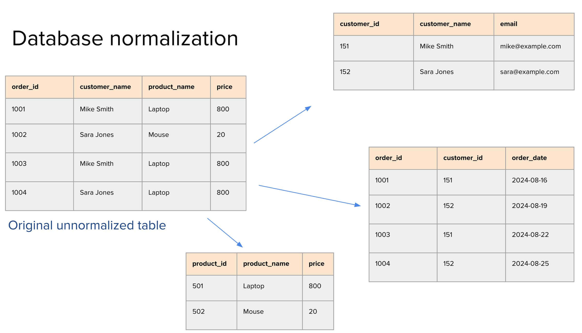
Imagine a table that records customer orders. It has four columns: order_id, customer_name, product_name, and price. Right away, you can spot inefficiencies. "Mike Smith" shows up more than once, and so does the product "Laptop." This redundancy means updates (e.g., changing Mike’s email or updating a laptop’s price) have to be made in multiple places, increasing the risk of inconsistency.
To fix this, we break the data into several normalized tables:
Customers: Contains unique entries for each customer with their customer_id, name, and email.
Products: Stores product_id, product_name, and price, again ensuring no repetition.
Orders: Links everything together using order_id, customer_id, and order_date.
By linking tables through IDs, we avoid duplicating information. This improves integrity, makes updates easier, and keeps storage efficient.
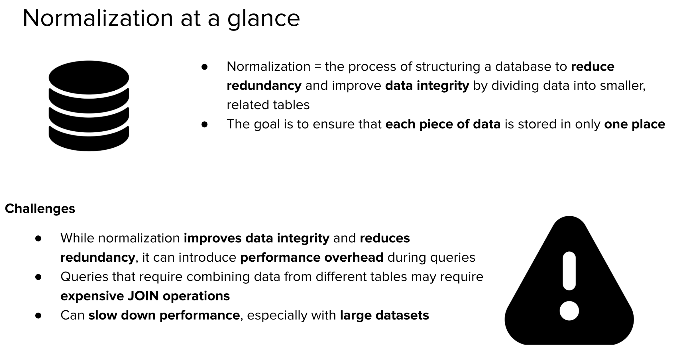
While normalization improves consistency, it introduces performance overhead during queries. Pulling a single view often requires JOINs across multiple tables. This can become expensive and slow, especially as datasets grow.
For example, retrieving order details with customer names and product prices might require a multi-table JOIN:
SELECT o.order_id, c.customer_name, p.product_name, p.price
FROM Orders o
JOIN Customers c ON o.customer_id = c.customer_id
JOIN Products p ON o.product_id = p.product_id;
With small datasets, this isn't a problem. But with millions of records, JOINs can become a bottleneck.
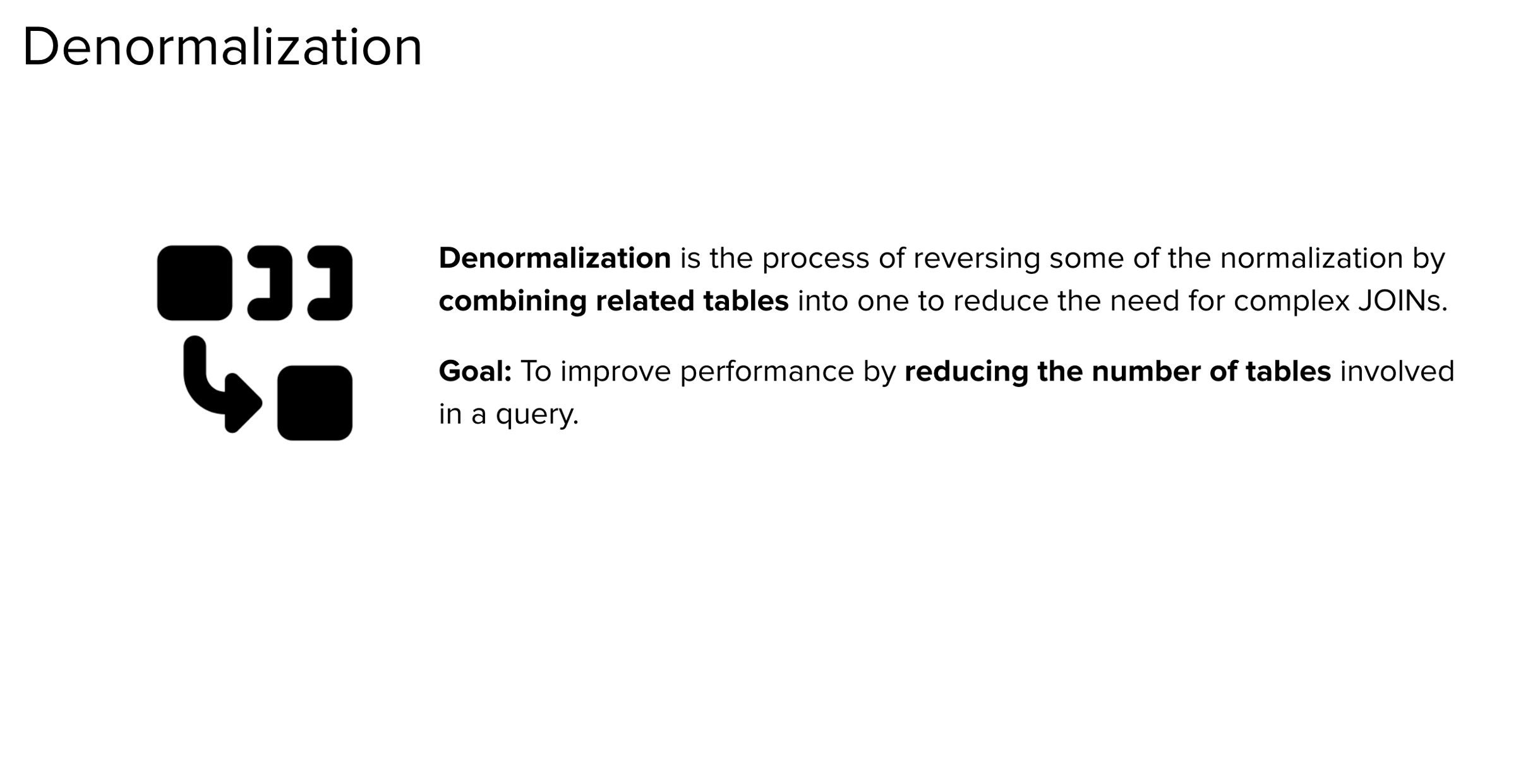
Denormalization is the process of combining related tables into one. Instead of splitting data across several tables, you keep related information together, even at the cost of some redundancy.
The main advantage? Simpler and faster queries. You reduce or eliminate JOINs, which are often the most performance-intensive part of SQL queries.
But there’s a trade-off. Denormalized tables often duplicate data, which can make updates harder and increase storage usage. If a store name changes, for example, you now have to update every row where that name appears.
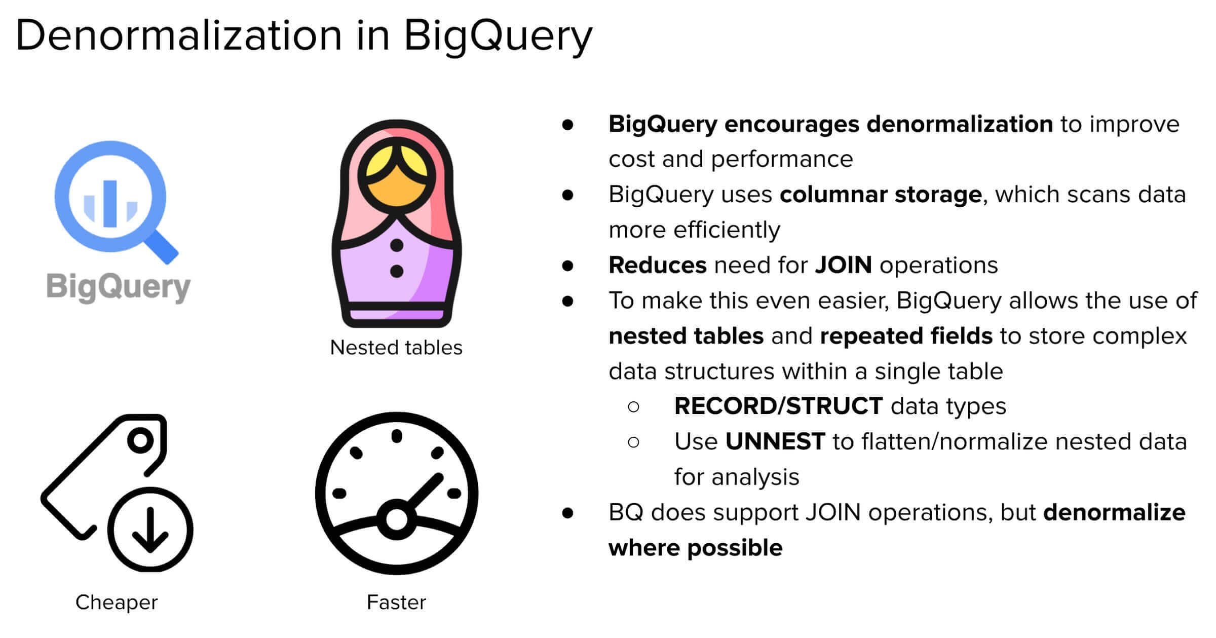
BigQuery flips the traditional conversation. Unlike many relational databases that strongly favor normalization, BigQuery encourages denormalization to improve both cost and performance.
Why? Several reasons:
Columnar Storage: BigQuery stores data by column, not row. This means it can scan only the columns needed for a query, making reads more efficient, even if the table is large and wide.
Minimized Need for JOINs: JOINs in BigQuery are expensive because they involve scanning and shuffling large datasets. Denormalization helps avoid this.
Nested and Repeated Fields: BigQuery supports complex types like STRUCT (nested records) and ARRAY (repeated fields), letting you pack related data into a single row. This is especially powerful for hierarchical data.
For example, consider this public weather dataset where each row represents a geographical point. Instead of storing hourly forecasts in a separate table, the forecast data is nested within each row. Each row contains an array of forecasted values for that point, one per hour.
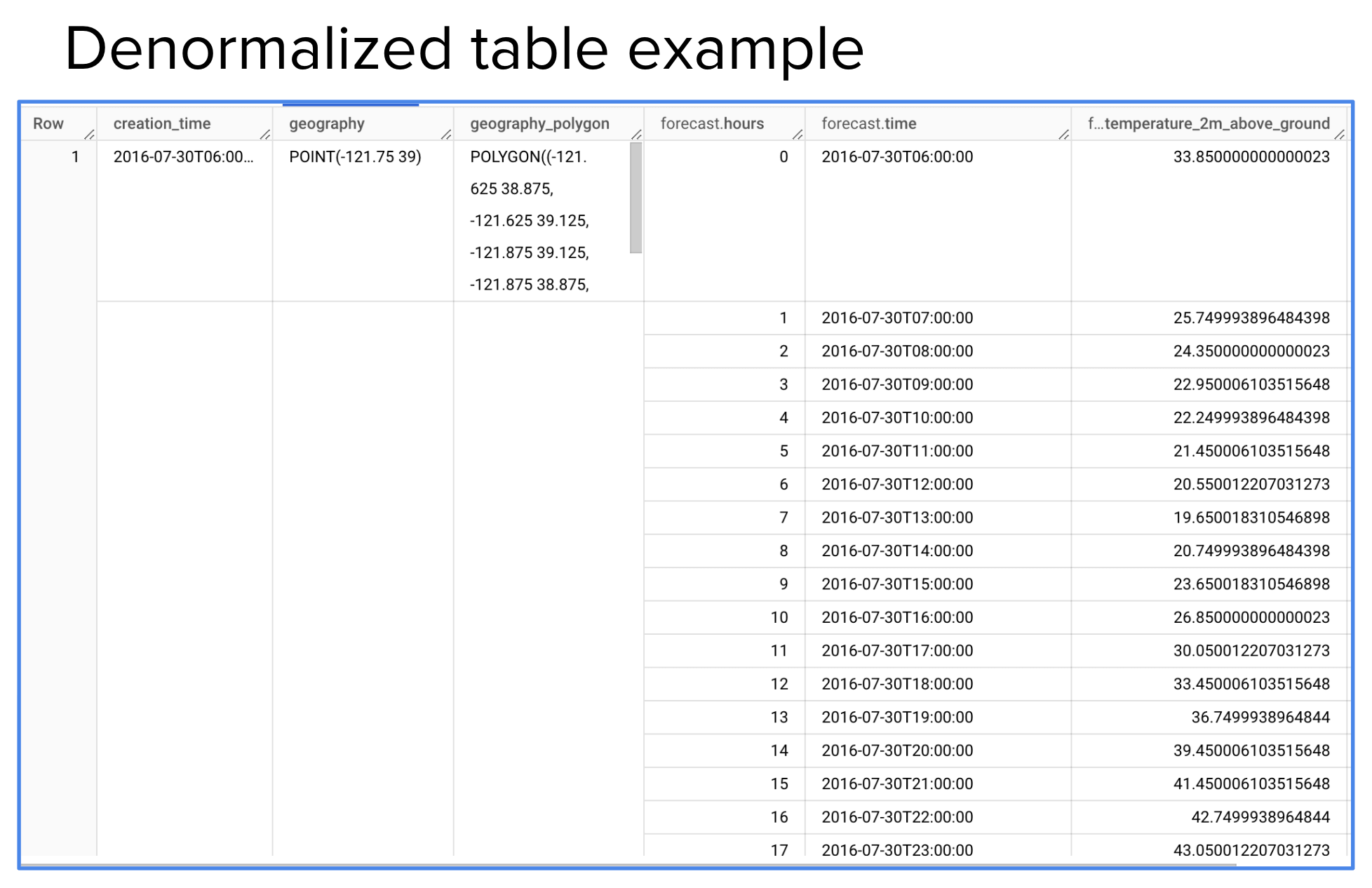
This structure allows queries like:
SELECT geography, forecast.time AS forecast_time, forecast.temperature_2m_above_ground AS temperature
FROM `bigquery-public-data.noaa_global_forecast_system.NOAA_GFS0P25`,
     UNNEST(forecast) AS forecast
WHERE forecast.hours = 10;
Using UNNEST, you flatten the nested data to extract temperature at a specific hour, without requiring joins. This structure keeps related data together while enabling flexible queries.
Let’s say you're building a system to analyze temperature forecasts for different locations. You can either:
Normalize the data: One table for locations, another for hourly forecasts, linked by a location_id.
Denormalize the data: Store all hourly forecasts as a nested array inside a single table row for each location.
In BigQuery, the second approach is usually better. Columnar storage and nested fields allow you to scan just the temperature data for the required hour and location, without needing to shuffle data across tables. This results in cheaper and faster queries.
Despite BigQuery’s tilt toward denormalization, there are situations where normalization still makes sense, even in BigQuery.
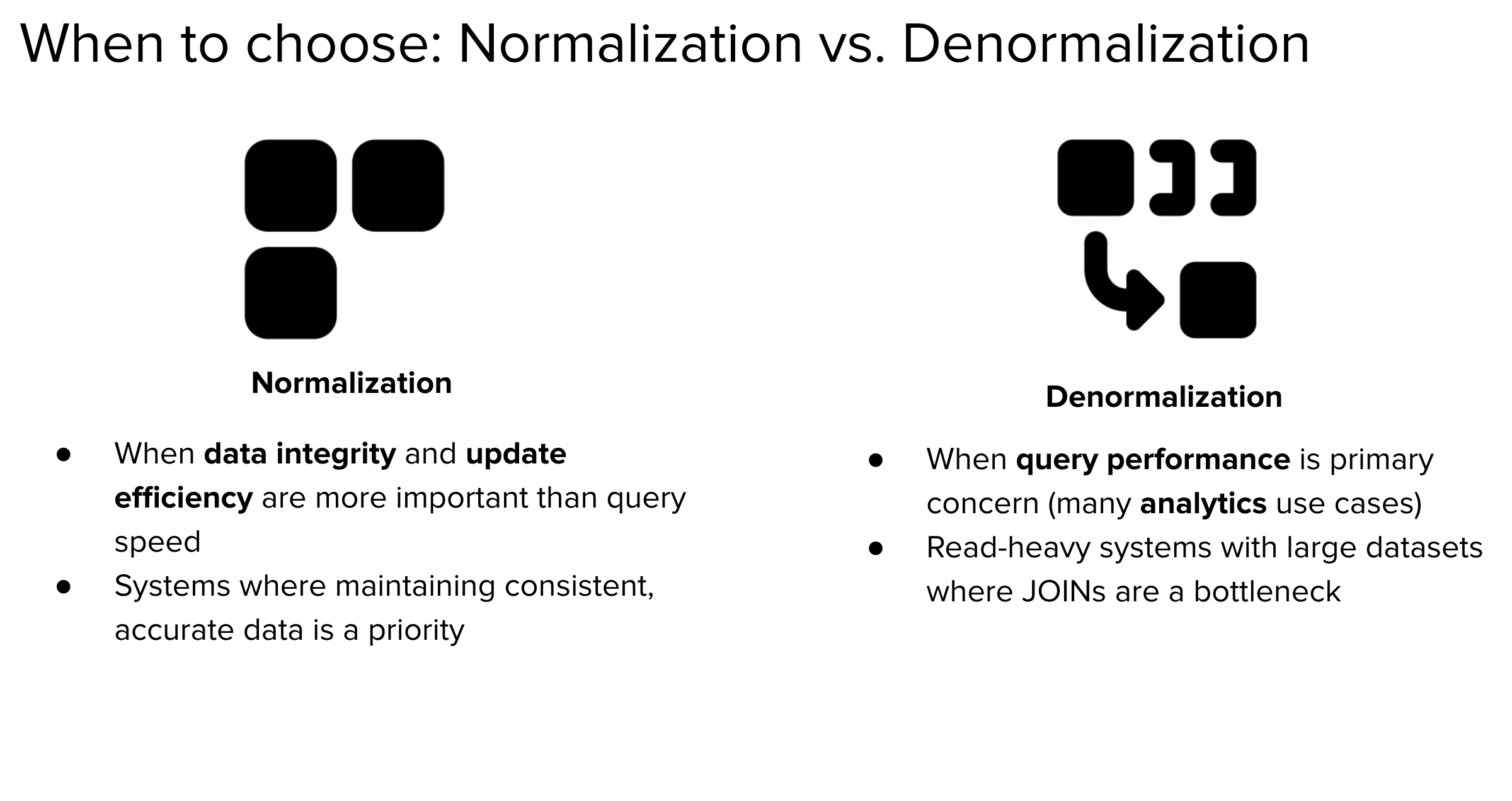
Use normalization when:
Data integrity is critical
You frequently update reference data (e.g., store locations or customer contact info)
You need to avoid redundant updates across massive tables
Consider a retail company with millions of transactions. The store's address or contact details might change occasionally. If you've denormalized store info into every transaction record, each update requires rewriting millions of rows. That’s expensive and error-prone.
Instead, you can keep a separate Stores table and reference it in the TransactionLogs table using a store_id. This structure supports efficient updates with minimal risk of inconsistency.
This kind of scenario might appear on a GCP certification exam:
You're designing a BigQuery data model for a retail company. There’s one table for store details and another for transaction logs. The company frequently updates store details and wants to maintain data integrity. What’s the best design?
The answer: Normalize the data. Keep store information in a separate table and link it using a store_id. This ensures updates are efficient and avoids having to touch millions of transaction rows.
Even though BigQuery supports denormalization, normalization is more appropriate when:
Updates are frequent
Redundant writes are costly
You need to enforce consistent data
| Criteria | Normalize | Denormalize |
|---|---|---|
| Data integrity | High priority | Less enforced |
| Update frequency | Frequent updates | Rare updates |
| Query performance | Moderate to poor with joins | Excellent with fewer joins |
| Dataset size | Small to large | Large, read-heavy datasets |
| Tool preference | Traditional RDBMS | BigQuery, analytics systems |
| Schema complexity | More tables, more joins | Fewer tables, nested structures |
Ultimately, it's not a binary decision. Good data engineering means knowing when to use each strategy. BigQuery gives you the flexibility to choose, based on your specific needs.
The key is to understand the trade-offs and align your schema design with the real-world behavior of your system, how often the data changes, how it’s queried, and how much scale you expect.
In BigQuery, denormalization is often the default. But with the right use case, normalization still has a valuable role to play.

